
Valuation, Demystified - Part 2
In Part 1 of our series on valuation, we established that we think about valuation in terms of expected return, and proposed the following formula:
Expected Return = Dividend Yield + Growth + Change in Valuation
An investor’s expected return is based on the cash flow received compared to price, the growth of that cash flow, and what another investor might be willing to pay for the same asset in the future. Part 2 of our series on valuation focuses on the importance of opportunity cost and how we think about future changes in valuation.
Opportunity Cost in Theory
What is a “good” expected return? The practice of investing involves choosing the best option among many choices. In this way, it is a comparative art. We think that the most logical standard for making this choice is expected rate of return.
“When an individual is confronted with investment opportunities across many different asset classes – for example, art, real estate, precious metals, private businesses, or public securities – the only way in which to make comparisons… is rate of return. It is the only standard by which all can be measured!” Chuck Akre
The best option among the choices that you don’t choose is called your “opportunity cost”. This is simply what you are giving up by choosing your first choice. It is by this standard (your next best alternative) that you should judge all investment decisions. Opportunity cost is sometimes referred to as a “discount rate” or “cost of capital,” but those are just fancy terms for the same idea. Charlie Munger summed opportunity cost up pretty well:
“If the new thing isn’t better than what you already know is available, then it hasn’t met your threshold.” Charlie Munger
This seems simple enough. In assessing whether something is a “good” investment or not, compare its expected return to that of your next best alternative.
However, in the real world there are thousands of next best alternatives available to every market participant. It would be practically impossible to keep track of an exhaustive list of the possibilities in order to benchmark each potential investment. What then is the solution?
Opportunity Cost in Practice
It makes sense to always have an objective yardstick of opportunity cost in your mind - one that you can easily calculate and apply on a daily basis as you consider making investments. Academics suggest that the right opportunity cost is the risk free rate of return (the interest rate you can earn on U.S. government bonds) adjusted for the risk of the investment as defined by the investment’s “Beta” (a measure of price volatility compared to the volatility of the market). We reject this definition of opportunity cost as unnecessarily obtuse and somewhat useless in practice. First, in today’s near-zero interest rate environment, how many investors are weighing whether to buy either Amazon stock or the ten-year treasury? Not many. Second, you would have a hard time finding any entrepreneur, business owner, or CEO who defined the riskiness of his or her business as it’s price volatility.
Instead, we think the most appropriate benchmark is a simple S&P 500 index fund - it’s readily available, practically free, and requires little to buy. Our argument is that the job of the active investor is to do at least better than expected rate of return of the S&P 500 over time, otherwise why bother? Buffett agrees:
“We think that the S&P annual [return] calculation has some meaning because it’s an alternative for people to invest. They don’t need us to buy the S&P. So unless, over time, we have some advantage over that, what are we contributing?” Warren Buffett
But what is the expected return of the S&P 500 and how is that return derived?
We can actually use our same expected return formula - involving price, earnings, ROE, and growth (and ignoring changes in valuation for now).
Expected Return = Dividend Yield + Growth
Expected Return = (Earnings x (1 - (Growth / ROE ))) / Price + Growth
Let’s start with price. For this we can just use a placeholder to keep it simple, say $100. We can then derive normalized earnings from this number by applying the historical average P/E ratio for the S&P 500:
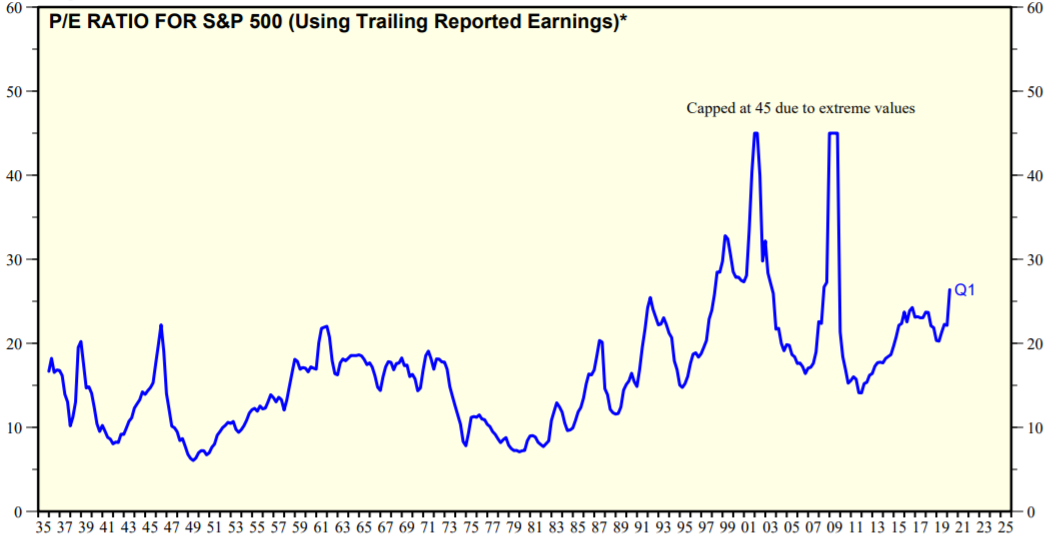
Source: Standard & Poor’s and Yardeni Research
As the P/E has averaged ~16x over time, we can say normalized earnings are ~$6.25 ($100 price / 16x multiple). We also know that the ROE of the S&P 500 has averaged ~13%.

Source: Standard & Poor’s and Semper Augustus Investment Group
What about growth? We can build out to expected distributable cashflow growth by starting with the metrics we know to be directionally correct. First, real GDP growth has averaged ~3% per year and inflation has averaged 1-2% per year, equating to 4-5% growth in nominal GDP. GDP growth is highly correlated with S&P 500 revenue growth:
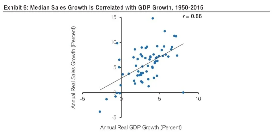
Source: Credit Suisse
So we can assume that S&P revenues also grow ~4.5% per year. Credit Suisse found that, on average, earnings tend to grow ~1.1x faster than revenue growth due to operating leverage, or the fact that some corporate costs are fixed:
“We measure operating leverage by examining the relationship between the change in sales and the change in operating profit in a particular period… The operating margin β is about 0.11... The way to interpret the β is that for every $1.00 change in sales, operating profit changes by approximately $0.11.” Credit Suisse
Based on this, S&P 500 earnings should grow ~5% per year, which is consistent with actual historical growth. We can assume that distributable cashflows grow in-line with earnings.
If we use our expected formula from earlier…
(Earnings x (1 - (Growth / ROE ))) / Price + Growth = Expected Return
($6.25 x (1 - (5% / 13%))) / $100 + 5% = 9%
We get an expected return for the S&P 500 of ~9%. So in summary, an active equity investor should demand at least a 9% return on any investment. That should be our yardstick.
A few side notes on this conclusion:
Another way to think about this is that the reason that the S&P trades at ~16x is precisely because investors have historically demanded a ~9% annual return.
Today, the S&P 500 trades at ~23x trailing operating earnings. That would imply an expected return of ~7.5%.
Conceivably, the expected return of the S&P 500 should decline if the opportunity cost of investing in the market (e.g. the risk free rate) is lower. During low interest rate environments, investors might only demanded a 7% return. This would only require a 2% dividend yield at the same level of growth. Using the numbers from above, a 2% dividend yield on $3.85 dividend ($6.25 x (1 - (5% / 13%)) would imply a $192.50 stock, or ~19x earnings of $10. This is a good explanation for why equity multiples tend to rise when interest rates fall.
Changes in Valuation
The fourth important source of expected return (after price, growth, and ROE) is the expected future change in valuation. We saved this for last because it is a somewhat ethereal concept. It is also “external” to the fundamentals of a business - it requires the market to act rationally, which is a tall order.
The “first principle” underlying why a specific valuation might change is, again, opportunity cost. Prices and thus valuations should theoretically change to normalize expected returns across different investment opportunities. In other words, an investment that implies a 15% expected return at a certain price should increase in price over time until the expected return normalizes to the ~9% opportunity cost of investing in the S&P.
Consider the example from Part 1 again: a stock costs $100 with earnings of $10, growth of 5%, and a 20% ROE.
($10 x (1 - (5% / 20%))) / $100 + 5% = Expected Return
7.5% + 5% = 12.5%
The expected return is 12.5%, above our 9% opportunity cost. In order to “normalize” the expected return to 9%, our example investment’s dividend yield would need to decrease to 4% at the current growth rate.
Expected Return - Growth = Dividend Yield
9% - 5% = 4%
As dividends are $7.50, the price would need to increase to ~$190.
Dividends / Dividend Yield = Price
$7.5 / 4% = $187.5
So, the valuation of this investment has increased from 10x ($100 price / $10 earnings) to 19x ($190 price / $10 earnings). Assuming this change happens over a period of say 10 years, that would represent an annual change of ~6.5% per year. So including this valuation change, the expected return of the investor paying $100 per share goes from 12.5% to 19%.
Dividend Yield + Growth + Change in Valuation = Expected Return
7.5% + 5% + 6.5% = 19%
One thing to take away is that as growth and ROE increase above market averages, the “fair” valuation required to normalize expected returns to opportunity cost increases as well. You can pay higher prices (and multiples) for above-average businesses because they will still generate expected returns commensurate with expected market returns.
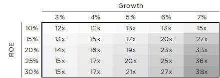
Source: Kaho Partners
We find this framework to be extremely useful when considering potential investment opportunities, in both the public and private markets. It provides a rough estimation of the returns we expect to make on a given investment, while also giving us a way to objectively benchmark those returns. However, the process - like any investment process - does require making predictions about the future, specifically about ROEs, growth rates, and valuation changes. Any process reliant on predictions is destined to be wrong, and it is our goal to limit our errors in ways that allow us to still achieve satisfactory results.
In Part 3, we discuss a few rules of thumb that we use to improve our chances of success.